
Weibull Blog
How to Perform a Weibull Analysis – Lifetime Distribution Selection and Parameter Estimation (Part 2 of 3)
Welcome to our three-part series about how to conduct a Weibull Analysis. In the first part, we discussed the preparation of life data and its importance in Weibull Analysis. Today, we will focus on lifetime distribution selection and parameter estimation.
Step 5: Lifetime Distribution Selection.
Statistical distributions were formulated by statisticians, mathematicians and engineers to mathematically model or represent certain behaviour. Those that can better represent life data is commonly called “lifetime distributions” or “life distributions“.
In Step 3, we collected as much relevant life data as practical. As was mentioned in the last post, good data, along with the appropriate model choice, usually results in good predictions. Thus, we need to choose the right lifetime distribution / life distribution that will fit the life data set and model the life of the component.
Types of Lifetime Distribution
Generally, we characterise life data model (i.e., lifetime distribution) by their failure rate, which refers to the chance of failing in the next small unit of time, given that the item operates that long.
Failure rates can be increasing (i.e., wear-out failure), decreasing (i.e., infant mortality or early failure), constant (i.e., useful life or random failure). In our future blog, we will discuss these failure patterns and their implications in detail.
Here is an overview of types of lifetime distribution:

How to Choose the Right Distribution: a theoretical method
If you have enough knowledge on the failure mechanism(s), extensive experience in Weibull Analysis, and have sufficient data in hand, you can use your engineering judgment to determine the right lifetime distribution. The following theoretical method can help guide the choice of distributions.
1) Look at the variable (data) in question.
- List everything you know about the conditions surrounding this variable (where it comes from, how was the data collected, how is it used, etc.)
- Use subject matter expert (SME) judgment (what do your engineers, materials, maintenance, operators, etc., know about the data)
2) Gather valuable information from historical data and analysis. Any particular distributions that have been previously used successfully for the same or a similar failure mechanism
3) Consult the literature for your industry to find examples of applications like yours. Look for a physical or statistical argument that theoretically matches a failure mechanism to a life distribution model
4) Review the descriptions and underlying assumptions of the probability distributions you are considering
5) Select the lifetime distribution that characterises this variable when the conditions and assumptions of the distribution match those of the variable.
How to Choose the Right Distribution: goodness-of-fit tests
When you are unsure of which lifetime distribution to use, you can perform goodness-of-fit (GOF) tests to determine the most appropriate model. Often, some Weibull Analysis software has the GOF feature to help.
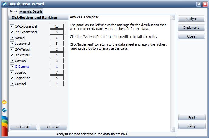
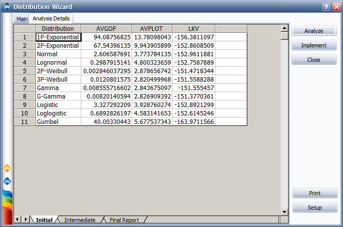
For example, the Distribution Wizard tool in ReliaSoft Weibull++ can help you identify which distribution provides the best math fit to your life data set. It uses three distribution fit tests to rank distributions (see images below):
- Kolmogorov-Smirnov test – AVGOF column: measures if the sample data comes from a specific distribution by evaluating the worst-case difference between the expected and obtained results.
- Normalized correlation coefficient test – AVPLOT column: measures how well the plotted points fit a straight line.
- Likelihood value test – LKV column: computes the value of the log-likelihood function, given the parameters’ fit of the distribution.
- Kolmogorov-Smirnov: the lower, the better the model fits your data.
- Likelihood Value: the higher, the better the model fits your data
- R-Squared Value: the higher, the better the model fits your data
A Summary of Different Types of Lifetime Distribution
- Weibull
- Lognormal
- Exponential
- Normal
- Generalised Gamma
- Logistic
- Gumbel
- 1-Parameter Weibull
- Weibull Bayesian
- Mixed Weibull
- Competing Failure Modes
When to Use
Increasing, decreasing or constant failure rate, or Monotonic
Application Comments
Appropriate to use in most cases where the probability of occurrence changes with time. One of the reasons for the popularity of the Weibull distribution is that it includes other useful distributions as special cases or close approximations, based on the value of the shape parameter, 𝛽.
Increasing failure rate
Application Comments
Useful for modelling naturally occurring variables. Used to model fatigue, corrosion and degradation type failure modes, and repair data.
Constant failure rate
Application Comments
Assumption of a constant instantaneous failure rate (or units that do not degrade with time or wear out), meaning that within a given time interval all items have the same probability of failing. (Time independent failures.) Often used on electronic components.
Increasing failure rate
Application Comments
It extends over the entire range of real numbers (from -infinity to +infinity) so it may be inappropriate to use for reliability. Useful for modelling the lifetimes of consumable items, such as printer toner cartridges.
When to Use
Increasing, decreasing or constant failure rate
Application Comments
Often used in meteorology and risk analysis. It is a distribution that can mimic others such as the Weibull or lognormal, based on the values of the distribution’s parameters. It should not be used with few failures.
Increasing failure rate
Application Comments
When results are driven by the products of several factors. Commonly applied in demographic and economic modelling because it is similar to the Normal distribution (i.e., bell shaped).
Max/Min analysis
Application Comments
Extreme value distributions model the maximum, or minimum, of a set of random variables. Engineers are interested in extreme values of a parameter (like minimum strength, maximum impinging force) because those values determine whether a system will potentially fail. It could be appropriate for modelling the life of products that experience very quick wear out after reaching a certain age.
When failure data is not available
Application Comments
Needs assumption of beta parameter, 𝛽; either from historical or similar product data.
Few failures and historical data available
Application Comments
Used to increase confidence of estimates when analyzing small data sets. Good historical data and some prior knowledge for the shape parameter are needed.
When multiple failure modes are present
Application Comments
Apply when responsible failure modes are not known. No root cause analysis (RCA) has been conducted.
When multiple failure modes are present
Application Comments
Apply when responsible failure modes are known. Root cause analysis (RCA) has been completed and failure modes have been identified for each failure.
Weibull
When to Use
Increasing, decreasing or constant failure rate, or Monotonic
Application Comments
Appropriate to use in most cases where the probability of occurrence changes with time. One of the reasons for the popularity of the Weibull distribution is that it includes other useful distributions as special cases or close approximations, based on the value of the shape parameter, 𝛽.
Lognormal
Increasing failure rate
Application Comments
Useful for modelling naturally occurring variables. Used to model fatigue, corrosion and degradation type failure modes, and repair data.
Exponential
Constant failure rate
Application Comments
Assumption of a constant instantaneous failure rate (or units that do not degrade with time or wear out), meaning that within a given time interval all items have the same probability of failing. (Time independent failures.) Often used on electronic components.
Normal
Increasing failure rate
Application Comments
It extends over the entire range of real numbers (from -infinity to +infinity) so it may be inappropriate to use for reliability. Useful for modelling the lifetimes of consumable items, such as printer toner cartridges.
Generalised Gamma
Increasing, decreasing or constant failure rate
Application Comments
Often used in meteorology and risk analysis. It is a distribution that can mimic others such as the Weibull or lognormal, based on the values of the distribution’s parameters. It should not be used with few failures.
Logistic
Increasing failure rate
Application Comments
When results are driven by the products of several factors. Commonly applied in demographic and economic modelling because it is similar to the Normal distribution (i.e., bell shaped).
Gumbel
Max/Min analysis
Application Comments
Extreme value distributions model the maximum, or minimum, of a set of random variables. Engineers are interested in extreme values of a parameter (like minimum strength, maximum impinging force) because those values determine whether a system will potentially fail. It could be appropriate for modelling the life of products that experience very quick wear out after reaching a certain age.
1-Parameter Weibull
When failure data is not available
Application Comments
Needs assumption of beta parameter, 𝛽; either from historical or similar product data.
Weibull Bayesian
Few failures and historical data available
Application Comments
Used to increase confidence of estimates when analyzing small data sets. Good historical data and some prior knowledge for the shape parameter are needed.
Mixed Weibull
When multiple failure modes are present
Application Comments
Apply when responsible failure modes are not known. No root cause analysis (RCA) has been conducted.
Competing Failure Modes
When multiple failure modes are present
Application Comments
Apply when responsible failure modes are known. Root cause analysis (RCA) has been completed and failure modes have been identified for each failure.
Other Considerations During Lifetime Distribution Selection:
- Whatever method is used to choose a lifetime distribution, the distribution should:
- Make sense – e.g., don’t use an exponential distribution with a constant failure rate to model an “Infant Mortality” failure mechanism.
- Pass visual and statistical tests for fitting the data
- The reliability engineer should have a practical justification for using a particular lifetime distribution. For example, the lognormal and the Weibull distribution are very flexible, therefore, sometimes both can fit a small set of failure data equally well. However, these two distributions may predict failure rates differently due to orders of magnitude.
Step 6: Parameter Estimation
In order to fit a statistical model to a life data set, the next step we need to conduct is to estimate the parameters of the lifetime distribution that will make the function most closely fit the life data set.
Before diving in the methods of parameter estimation, let’s firstly talk about a basic statistical term – probability density function and 3 parameter types.
Probability density function (PDF)
In Step 5, we selected the best-fit lifetime distribution to describe our life data set. Each type of life distribution has its own PDF to describe the distribution in a mathematical or visual way.

Types of parameters – Shape, Scale, and Location parameters
Distributions can have any numbers of parameters. The number and values of the parameters of a lifetime distribution can directly affect the distribution characteristics, both in the reliability metrics and in the visual demonstration (i.e., representing PDF on a plot).
In general, the lifetime distributions used for reliability and life data analysis are usually limited to a maximum of three parameters. These three parameters are usually known as the scale parameter, the shape parameter, and the location parameter.
- Scale Parameter: defines where the bulk of the lifetime distribution lies, or how stretched out the distribution is. It is the most common type of parameter. In 1-parameter distributions, the only parameter is the scale parameter.
- Shape Parameter: defines the shape of a lifetime distribution. Distributions, like the exponential or normal, do not have a shape parameter since they have a predefined shape that does not change over time.
- Location Parameter: defines the location of the lifetime distribution in time. It is usually denoted as γ, which can be either positive or negative.
The Effect of Parameters on the Distribution
We will take a 3-parameter Weibull distribution as an example to visually demonstrate the effect of the values of parameters on a distribution (see image below). In Weibull distribution, β is the shape parameter (aka the Weibull slope), η is the scale parameter, and γ is the location parameter.

Parameter Estimation Methods
For any lifetime distribution, the parameter or parameters of the distribution are estimated (obtained) from the data that we have collected and classified.
In Step 4, we classify life data into 4 types: complete, right censored (suspended), Internal censored, and left censored data (see the image below). Different data type requires different analysis methods to estimate the parameters.

- Probability plotting
- Least squares (rank regression) estimation
- Maximum likelihood estimation (MLE)
- Bayesian Estimation Method
Drawbacks:
- Require lots of effort
- High risk of inaccurate results
It has 2 types: for rank regression on Y (RRY), the sum of squares of the vertical deviations is minimized; for rank regression on X (RRX), the sum of the squares of the horizontal deviations is minimized.
Drawbacks:
- Time-consuming, especially when there are lots of parameters need to be estimated
- Requires sufficient data
- Difficult to determine the “best fit” model
A method that requires reliability engineers to incorporate prior knowledge and information, along with a given set of current observations, to make parameter estimation.
Bayesian estimation method can be particularly useful when there is limited test data for a given failure mode but there is a strong prior understanding of the failure rate behaviour for that mode.
Probability plotting
Drawbacks:
- Require lots of effort
- High risk of inaccurate results
Least squares (rank regression) estimation
It has 2 types: for rank regression on Y (RRY), the sum of squares of the vertical deviations is minimized; for rank regression on X (RRX), the sum of the squares of the horizontal deviations is minimized.
Maximum likelihood estimation (MLE)
Drawbacks:
- Time-consuming, especially when there are lots of parameters need to be estimated
- Requires sufficient data
- Difficult to determine the “best fit” model
Bayesian Estimation Method
A method that requires reliability engineers to incorporate prior knowledge and information, along with a given set of current observations, to make parameter estimation.
Bayesian estimation method can be particularly useful when there is limited test data for a given failure mode but there is a strong prior understanding of the failure rate behaviour for that mode.
Rule of Thumb Regarding Parameter Estimation Methods
- Use Rank Regression (RRX): Complete data and small sample sizes
- Use MLE: Heavy and/or mixed censoring; Larger sample sizes (30+ failures)
Weibull Analysis Related Resources:
Blog:
- How to Perform a Weibull Analysis – Data Preparation (Part 1 of 3)
- How to Perform a Weibull Analysis – Lifetime Distribution Selection and Parameter Estimation (Part 2 of 3) [THIS BLOG]
- How to Perform a Weibull Analysis – Validation of Results and Reliability Improvement (Part 3 of 3)
- The Quick Guide to Perform a Weibull Analysis [one-page infographic]
Weibull Analysis Software: ReliaSoft Weibull++ – Provide the most comprehensive toolset (e.g., distribution wizard) available for reliability life data analysis, calculated results, plots and reporting.
Subscribe to our newsletter to stay up-to-date! If you need any advice/ training on Weibull Analysis, our team at HolisticAM are here to help! Contact us 📞
