
How to Perform a Weibull Analysis – Validation of Results and Reliability Improvement (Part 3 of 3)
Welcome to part three of our three-part series about how to conduct a Weibull Analysis. In the last two posts, we discussed how to gather life data set, select the best-fit lifetime distribution, and estimate the parameters that will fit the distribution to the data.
Today we will cover the final steps of a Weibull Analysis:
- Step 7: Generate plots and calculate the functions of certain distribution
- Step 8: Indicate Confidence Bounds – estimate the precision of an estimate
- Step 9: Review the Analysis in 4 aspects: practical, graphical, analytical, and confidence
- Step 10: Determine and implement appropriate strategies
Ready? Let’s dive in!
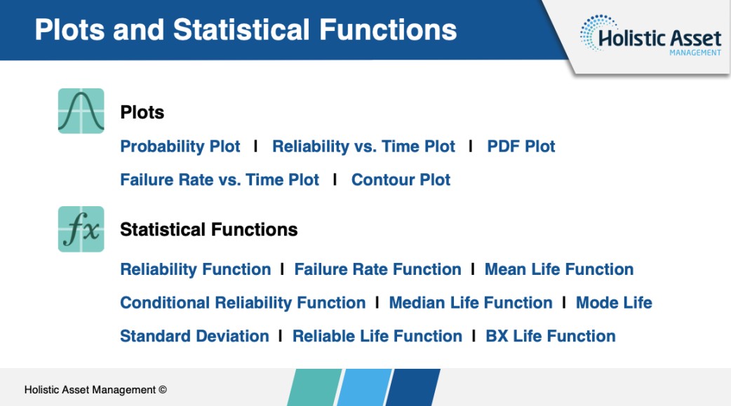
Step 7: Generate Plots and Calculate Statistical Functions
You’ve selected the right lifetime distribution and have estimated the parameters to fit that distribution to a particular life data set. Now it’s time to generate plots and calculate a variety of statistical functions from the analysis (see image below).
Basic Statistical Background
Before having a detailed explanation of these reliability and life data metrics, let’s talk about the basic statistical background in reliability analysis:
[1] T, the failure time (aka time-to-failure of a component), is a continuous random variable with a known distribution. Since the component can be found failed at any time after time 0, T value can range from 0 to infinity.
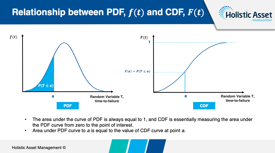
[2] f(t) (i.e. Probability Density Function, PDF) represents the relative frequency of failure times as a function of time.
- Each lifetime distribution has its own predefined f(t), once you estimate the parameters based on the life data set (step 6), the f(t) is completely defined so that you can obtain any value for f(t) given any value of t.
- We also mentioned in the last post that PDF is the basis for almost all of other important reliability and life data functions.
[3] F(t) (i.e., Cumulative Distribution Function, CDF) measures the cumulative probability that the component under observation will fail before the associated time value, t. It is also known as the unreliability function, represented by Q(t).
Statistical Functions
- Reliability Function
- Failure Rate Function
- Conditional Reliability Function
- Mean Life Function
- Median Life Function
- Mode Life Function
- Reliable Life Function
- BX Life Function
- Provides the probability of success, or the probability of not observing a failure, by time t.
- Also known as Survival function, represented by S(t)

Note: Reliability should be specified with an associated time; in other words, it is incorrect to say that the reliability is 90% without saying at what time. i.e. 90% reliability at 7 months. To be more complete, one should always specify reliability by specifying reliability, time and confidence level.
- Provides the number of failures occurring per unit time. Failure rate is denoted as failures per unit time.
- Also known as Hazard Rate Function, when discussing a non-repairable system. Represented by H(t).
- Mathematically:

- It is useful in characterising the failure behaviour of a component, determining maintenance crew allocation, planning for spares provisioning, etc.
Note: The failure rate is constant only for the exponential distribution; in most cases the failure rate changes with time.
- Provides the probability of a component successfully completing a new mission of t duration, given that it has already successfully completed a mission of T duration.
- Mathematically:

- It is a useful metric when you are using BlockSim‘s QCP to compute the conditional reliability of a system.
- Provides a measure of the average time of operation to failure.
- Also known as Mean Time-to-Failure (MTTF)
- Mathematically:

Tips: People always refer to MTTF as the MTBF (Mean Time Between Failures). This is not correct for most cases. The only time that the MTTF is the same as the MTBF is if the failure rate is constant, an assumption that is often questionable. Generally, MTTF should be used for non-repairable systems and MTBF should be used for repairable systems.
Note: The MTTF cannot be the sole measure of the reliability of a component because different distributions may have identical means.
- The failure time(s) that has exactly one-half of the area under the PDF to its left and one-half to its right.
- Mathematically,

- Symmetric distribution has only one median, while asymmetric distribution had two.
Note: Many people use mean and median interchangeably. This is incorrect, as the mean and median have the same values only when it is a symmetric distribution. In some cases, there can be a large difference in the values of the median and the mean.
- Also known as Modal Life Function.
- The maximum value of t that satisfies

- For a continuous distribution, the mode is the t value that corresponds to the maximum probability density (i.e., the value where the PDF has its maximum value, namely the peak of the PDF curve).
- The estimated time when the reliability will be equal to a specified goal.
- Useful in estimating warranty time.
- For example, the estimated time of operation is 4 years for a reliability of 90%.
- Provides the time at which X% of the population is expected to fail, or the time for corresponding unreliability of X%.
- Mathematically,

- For example, if 5% of the products will fail by 2 years of operation, then the B(5) life is 2 years. It is equal to a reliable life of 2 years for a 95% reliability.
Reliability Function
- Provides the probability of success, or the probability of not observing a failure, by time t.
- Also known as Survival function, represented by S(t)
Note: Reliability should be specified with an associated time; in other words, it is incorrect to say that the reliability is 90% without saying at what time. i.e. 90% reliability at 7 months.
Failure Rate Function
- Provides the number of failures occurring per unit time. Failure rate is denoted as failures per unit time.
- Also known as Hazard Rate Function, when discussing a non-repairable system. Represented by H(t).
- Mathematically:
- It is useful in characterising the failure behaviour of a component, determining maintenance crew allocation, planning for spares provisioning, etc.
Note: The failure rate is constant only for the exponential distribution; in most cases the failure rate changes with time.
Conditional Reliability Function
- Provides the probability of a component successfully completing a new mission of t duration, given that it has already successfully completed a mission of T duration.
- Mathematically:
- It is a useful metric when you are using BlockSim‘s QCP to compute the conditional reliability of a system.
Mean Life Function
- Provides a measure of the average time of operation to failure.
- Also known as Mean Time-to-Failure (MTTF)
- Mathematically:
Tips: People always refer to MTTF as the MTBF (Mean Time Between Failures). This is not correct for most cases. The only time that the MTTF is the same as the MTBF is if the failure rate is constant, an assumption that is often questionable. Generally, MTTF should be used for non-repairable systems and MTBF should be used for repairable systems.
Note: The MTTF cannot be the sole measure of the reliability of a component because different distributions may have identical means.
Median Life Function
- The failure time(s) that has exactly one-half of the area under the PDF to its left and one-half to its right.
- Mathematically,
- Symmetric distribution has only one median, while asymmetric distribution had two.
Note: Many people use mean and median interchangeably. This is incorrect, as the mean and median have the same values only when it is a symmetric distribution. In some cases, there can be a large difference in the values of the median and the mean.
Mode Life Function
- Also known as Modal Life Function.
- The maximum value of t that satisfies
- For a continuous distribution, the mode is the t value that corresponds to the maximum probability density (i.e., the value where the PDF has its maximum value, namely the peak of the PDF curve).
Reliable Life Function
- The estimated time when the reliability will be equal to a specified goal.
- Useful in estimating warranty time.
- For example, the estimated time of operation is 4 years for a reliability of 90%.
BX Life Function
- Provides the time at which X% of the population is expected to fail, or the time for corresponding unreliability of X%.
- Mathematically,
- For example, if 5% of the products will fail by 2 years of operation, then the B(5) life is 2 years. It is equal to a reliable life of 2 years for a 95% reliability.
Step 8: Indicate Confidence Bounds
Given the limitation of time and resources, we can only select relatively small but representative samples of units to understand the life characteristics of all products (i.e. the probability of failure) in the population. To quantify the uncertainty due to sampling error, we use Confidence Bounds (aka Confident Interval) to estimate the precision of an estimation.
The Confidence Bound gives an estimated range of values that is likely to include an unknown population parameter. It is calculated from the set of sample life data.
1-sided and 2-sided Confidence Bounds
- 1-sided confidence bounds: One-sided bounds are used to indicate that the quantity of interest is above the lower bound or below the upper bound with a specific confidence.
- 2-sided confidence bounds: Two-sided bounds are used to indicate that the quantity of interest is contained within the bounds with a specific confidence.
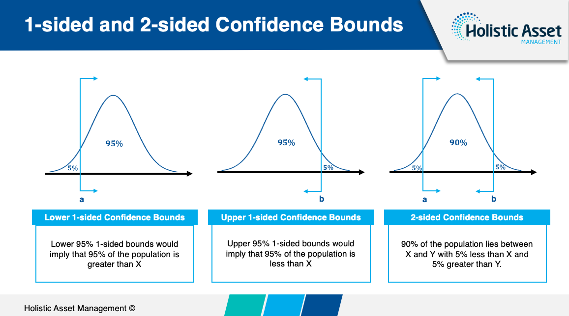
Tips:
The appropriate type of bounds depends on the application.
- 1-sided lower bound on reliability;
- 1-sided upper bound for percent failing under warranty;
- 2-sided bounds on the parameters of the distribution;
Confidence Bounds Methods
In this post, we just list the methods of calculating Confidence Bounds. If you want to review the methodologies comprehensively, read the “Confidence Bounds” chapter in ReliaSoft Weibull Analysis eTextbook.
(1) Fisher Matrix Confidence Bounds (FM): These bounds are employed in many statistical and life data analysis packages, as well as most ReliaSoft applications. In general, these bounds tend to be more optimistic (tighter) than the non-parametric beta-binomial or likelihood ratio bounds.
(2) Beta Binomial Confidence Bounds (BB): A non-parametric approach to confidence interval calculations involves the use of rank tables.
(3) Likelihood Ratio Confidence Bounds (LR): LR and FM are both commonly used in Weibull Analysis to calculate reliability confidence bounds for different life distributions. Here are the differences between LR and FM:
- LR is much simpler than FM.
- LR is computationally intensive and needs a much longer time to plot.
- LR is more conservative than those calculated with the FM method.
- FM relies on a normality assumption, while LR relies on the assumption that follows a Chi-Square distribution.
(4) Bayesian Confidence Bounds (BSN): Can be used when one has some prior knowledge about the reliability of the component with adequate historical data and/or engineering judgment.
Order of Preference for Confidence Bound Methods for Small Samples: BSN > LR > FM >BB
The SimuMatic tool in Weibull++ can be used to perform many reliability analyses on data sets that have been created using Monte Carlo simulation.
Functions:
- Better understand life data analysis concepts
- Experiment with the influences of sample sizes and censoring schemes on analysis methods
- Construct simulation-based confidence bounds
- Better understand the concepts behind confidence bounds
- Design reliability tests
Display confidence bounds on time (Type I) or on reliability (Type II)
When drawing a probability plot, confidence bounds (except Beta Binomial Confidence Bounds) can be displayed in two ways: 1) on time (Type I) or 2) on reliability (Type II). Type I is to read values from the x-axis (time), while Type II is to read values from the y-axis (probability of failure).
The rule of thumb is: display confidence bounds on the value that you do not know (i.e., the value that you are trying to estimate).
- Type I: given an unreliability value, what is the corresponding time? For example, if you want to determine the time by which 8% of the units have failed (i.e. 92% reliability) then you would use confidence bounds on time.
- Type II: given a time value, what is the corresponding unreliability? For example, if you want to determine the probability of failure at 1500 hours, then you would use confidence bounds on reliability.
Step 9: Analysis Review
Before taking actions, you need to review the entire Weibull Analysis. Basically, you should consider 4 aspects: Practical, Graphical, Analytical, and Confidence.
Practical
In terms of the practical aspect, ask yourself:
- Does the data show trends or clues that are of practical importance?
- What does your in-house subject matter expert think about the data based on their expert and previous experience?
- Is the variation in data associate with some outside influences such as:
- changes from shift-to-shift,
- weather related variation caused by temperature or humidity,
- part-to-part variation (items may not be identical due to new models or versions).
Graphical
In terms of the graphical aspect, ask yourself:
- Are your data points reasonably spaced along the line, or are some points far from the line?
- Does your Weibull plot contain an “S” or “dogleg” bend in the data? (it is a clue to the potential of multiple failure modes, which means you need to have a more diligent review)
- Does your Weibull plot appear to curve downward at early life? (it is a clue that your assumption of origin time might be incorrect. Time does not start at T=0. It may be physically impossible for the failure mode to produce failures instantaneously, or at early life.)
Analytical
In terms of the analytical aspect, ask yourself:
- Are your Rho (ρ) or Likelihood values too low? (it means your data collection might have some issues.)
- Do the parameters match expectations? (In Weibull distribution if the slope is too high it may be an indication of poor data sampling, you may have a very narrow window of extreme use.)
- Can you apply historic information to improve your estimate? (One common way to do this is to impose a known Weibull slope based on multiple test results that engineering judgement has determined to best represent the failure mode under study.)
Confidence
In terms of the confidence aspect, ask yourself:
- Is the confidence bound adequate to cover the variation risk?
- Are there any outliers that lie an abnormal distance from other values? Why do they appear? After eliminating them, how likely it is that similar values will continue to appear? (remember, always document the justification and subsequent removal of any outliers)
- Is the width of the confidence bound reasonable? (A very wide interval may indicate that more data should be collected before anything very definite can be said about the parameter)
Step 10: Determine and Implement Appropriate Strategies
Now you have everything you need to understand the life characteristics of all products in the population, what do you then do with these results? What actions do you take to improve the reliability and cost performance of products?
Choose the Optimal Strategies based on Beta Value, β
You can determine the best maintenance strategies based on the types of the failure patterns of the component, which are represented by the beta value, β. The beta value is simply a measure of the slope of the probability plot.
The “Reliability Bathtub Curve” in the Failure Rate vs Time plot (see image below) is a graphical representation that comprises all of the 3 failure patterns: infant mortality failures (β <1) with a decreasing failure rate, random failures (β = 1) with a low, relatively constant failure rate, and wear-out failures (β >1) that shows an increasing failure rate.

- Inadequate quality assurance and control in design
- Inadequate quality assurance and control in manufacturing
- Lack of burn-in or stress testing
What to Do About It?
- Choose the best design approaches, such as Appropriate specifications, adequate design tolerance and sufficient component derating.
- Start stress testing, such as HALT (Highly Accelerated Life Test) or HAST (Highly Accelerated Stress Test), at the earliest development phases to evaluate design weaknesses and detect specific assembly and materials problems.
- Apply stress testing in early production phases to precipitate failures to effectively identify defects, analysing the resulting failures and take corrective action through redesign to eliminate the root causes of these defects.
Stress exceeding strength such as human error during maintenance, induced failures, accidents and natural disasters.
What to Do About It?
- Conduct condition monitoring.
- If the failure is considered as unacceptable, redesign and replace the component or the system before it fails;
- If the cost of replacement outweighs the benefit gained from making changes, and the failure is not significant, leave it in operation, tackle it when the failure occurs.
- Fatigue or depletion of materials
- Corrosion or erosion
- Inherent failures of materials
- Accumulated damage
What to Do About It?
- If the failure is significate and rapid wear-out (i.e., β>4), overhauls may be the most cost-effective.
- If the failure is early wear-out (i.e., 1< β<4), preventative maintenance optimisation strategies may be the most cost-effective. Schedule optimal replacement or remediation maintenance strategies at a given time interval (can be determined by CDF) to avoid the failure before it occurs.
Infant Mortality Failures
- Inadequate quality assurance and control in design
- Inadequate quality assurance and control in manufacturing
- Lack of burn-in or stress testing
What to Do About It?
- Choose the best design approaches, such as Appropriate specifications, adequate design tolerance and sufficient component derating.
- Start stress testing, such as HALT (Highly Accelerated Life Test) or HAST (Highly Accelerated Stress Test), at the earliest development phases to evaluate design weaknesses and detect specific assembly and materials problems.
- Apply stress testing in early production phases to precipitate failures to effectively identify defects, analysing the resulting failures and take corrective action through redesign to eliminate the root causes of these defects.
Random Failures
Stress exceeding strength such as human error during maintenance, induced failures, accidents and natural disasters.
What to Do About It?
- Conduct condition monitoring.
- If the failure is considered as unacceptable, redesign and replace the component or the system before it fails;
- If the cost of replacement outweighs the benefit gained from making changes, and the failure is not significant, leave it in operation, tackle it when the failure occurs.
Wear-out Failures
- Fatigue or depletion of materials
- Corrosion or erosion
- Inherent failures of materials
- Accumulated damage
What to Do About It?
- If the failure is significate and rapid wear-out (i.e., β>4), overhauls may be the most cost-effective.
- If the failure is early wear-out (i.e., 1< β<4), preventative maintenance optimisation strategies may be the most cost-effective. Schedule optimal replacement or remediation maintenance strategies at a given time interval (can be determined by CDF) to avoid the failure before it occurs.
Run Simulation to Determine Your Optimal Strategies
Alternatively, you can use the Weibull results by putting the data into your RBD Blocks and running the full system simulation of a period of time, you will be able to accurately define the failure profile of the component and system, and forecast the best strategies to meet your reliability and cost needs.
Summary
Now that the process of performing a Weibull Analysis has been listed and discussed step-by-step. Starting from collecting life data to determining the type of distribution and estimating the parameters, followed by generating results and reviewing the analysis, and finally determining the appropriate strategies to improve reliability and cost performance.
In the next post, we will share you with a one-page infographic to visualise the whole process of how to perform a Weibull Analysis. Don’t miss out!
Weibull Analysis Related Resources:
Blog:
- How to Perform a Weibull Analysis – Data Preparation (Part 1 of 3)
- How to Perform a Weibull Analysis – Lifetime Distribution Selection and Parameter Estimation (Part 2 of 3)
- The Quick Guide to Perform a Weibull Analysis [one-page infographic]
Weibull Analysis Software: ReliaSoft Weibull++ – Provide the most comprehensive toolset available for reliability life data analysis, calculated results, plots and reporting.
Subscribe to our newsletter to stay up-to-date! If you need any advice/ training on Weibull Analysis, our team at HolisticAM are here to help! Contact us 📞
